Neural Networks Less Hard

An introduction to neural networks that anyone can understand

Goal: My goal for this tutorial is to teach you how neural networks (aka Deep Learning) work from basically nothing to a deep understanding, including the underlying mathematics.

Assumptions: The only pre-requisites I assume is that you have a high-school level mathematics background, basically meaning you can comfortably solve for $x$ in algebraic equations like $3x+5 = 11$ and understand functions like $f(x) = m*x + b$ and graph points on an X-Y plane. I will teach you all the rest. The only catch is that this is long and moves slowly. But if you follow along, you will understand and be able to do Deep Learning by the end.

Motivation: There are many books, tutorials and resources that teach deep learning and neural networks, but most of them make it way too complex. Neural networks are actually really simple fundamentally. Modern deep learning algorithms are complex but that’s only because they add a lot of fancy bells and whistles to what is actually a very simple function.

Note: Hover over highlighted words for additional information.

Neural networks are what power all the technology called artificial intelligence these days (such as ChatGPT). The category of modern neural networks are often referred to Deep Learning. Deep Learn algorithms (aka neural networks) can be used to predict what you’re going to type next in a text message, generate realistic images, drive cars, optimize energy usage in factories and many many other tasks; that’s what makes them so powerful.

Here is how neural networks are often first introduced and depicted in a tutorial:

Neural networks are often introduced by referencing their relationship to biological neural networks, where you have “neurons” (or nodes) connecting and sending information to other neurons in different “layers” via their connection “weights.” The fact that modern neural networks have multiple layers in series is where the “deep” in Deep Learning comes from.

Then training the neural network involves backpropagation, which involves sending error signals back through the neural network graph to update the weights of the network. Often this is depicted as an “error unit” sending an error signal back to the output layer, which sends its own error signal back to the prior layer and so on.

That is not an inaccurate depiction, but it tells you nothing about how to actually implement a neural network in code, and if you don’t know how to implement a neural network in code, you don’t understand neural networks.

Let’s demystify.

A neural network (aka Deep Learning) is a nested function.

What is a nested function? A nested function, also called a compositional function, is a function that has other functions inside of it. It’s like if you have a box inside of a box inside of a box inside of a box, where each box is a function. Now, I want to make this as accessible as possible, so let’s backup and define what a function is.

A function is a set of instructions that takes some input data and transforms it into a different form (the output data).

This is a fairly broad definition of a function. A function can therefore be as simple as a table like this:

Input	Output
00	11
01	10
10	01
11	00

The instructions for this function are just to find the input in this table and then the corresponding cell under the Output column is the output of this function. This is called a lookup table.

We could have defined a similar function using more operational instructions as opposed to a look up table. For example, we could have defined this function as: take each digit of the input number and flip it, so if a digit is a 0 then flip it 1 and if its a 1 then flip it to 0.

A few definitions are in order. A function transforms individual instances, or elements or terms or values (all equivalent terms) from a particular input space or set or type (all equivalent terms in this context) into new values of a potentially different output type. For example, the input type of our first binary function using the lookup table is the type of binary numbers of length 2, because that is only what our lookup table shows, and the output type is the same. The input type of our second more operationally defined function is the type of all binary numbers of any length, since it flips the individual digits of a binary number. A type can be thought of as a specification of a certain set of values that you want to define as a group. Another way to think of a type is as a constraint. Rather than letting a function consume any possible value (whether it be a number, or English characters, or something else) you define a type as a constraint on what is allowed as an input into and out of a function.

I like to think of functions like little machines where input material gets sent inside along a conveyor belt from the left and this input material gets transformed into some output material then gets sent out on the right side on another conveyor belt. This lends itself to a nice graphical view of functions, which are called string diagrams because it looks like they have little strings going in and out, representing data going in and coming out:

I also like to annotate the input and output types.

Okay, so now that we have a good idea of what a function is, let’s demystify a compositional function (aka nested function). A compositional function is just a function that is composed of multiple functions, and therefore can be decomposed into a set of separate functions that are applied in sequence. Let’s see this graphically.

Here I’ve defined two functions, Function 1 takes a binary number as an input and returns a new binary number as output, then it passes that value into Function 2, which transforms that binary number into some English letters like A, B, C, etcetera. I could keep these as just two separate functions, but if I package them together and give it a name, now we have a nested or compositional function.

In typical mathematical and programming notation, you would call this function like so: function2(function1(X)). First you apply function1 to X, and then apply function2 to the result of that.

And that is the essence of deep learning. The “deep” in Deep Learning is just about these kinds of compositional (or nested or sequential) functions. That’s basically it. Now obviously I’ve left out the details of what the composed functions actually do in a neural network, but even that is not too complicated. Let’s keep going.

A neural network looks just like the figure above, except we call each of those “inner” or composed or nested functions a layer, and each layer function takes a vector as an input and returns a new vector as an output.

A layer in a neural network is just a function that takes a vector and transforms it into a new vector.

Layer functions transform the input vectors by 1) multiplying them with a matrix and 2) applying a non-linear activation function. Again, to make this as accessible as possible, I’m going to assume you have no idea what vectors or matrices are, and have no idea what a “non-linear function” means.

But let’s start with a concrete problem to solve and work our way to an understanding of these concepts. We will do this by studying a non-deep learning problem.

Non-Deep (Shallow) Learning

Let’s say you are a climate scientist and you’ve collected some data about the global average DefinitionThe average, also called mean, of a set of numbers is the sum of the numbers divided by the total number of numbers. temperature over the past several decades.

The global mean temperature for a particular time period is the average temperature of Earth’s surface over that time period. To calculate it, meteorologists and climate scientists collect temperature data from thousands of weather stations on land, from sea vessels, and from satellites measuring atmospheric and surface sea temperatures. They then combine these readings to estimate the average temperature of the entire surface of the planet.

Here’s what the data looks like when graphed:

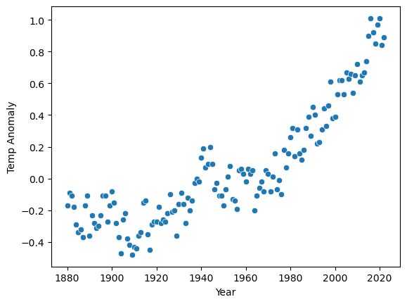
The x-axis is the year from 1880 to 2022 and the y-axis is the temperature anomaly, which is the difference in the global mean temperature for each year compared to the long-term average from 1951 to 1980. For example, if the average temperature for the years 1951-1980 was 14°C, and the global mean temperature for the year 1880 was 13.83°C (which is 0.17°C lower), then the temperature anomaly for 1880 would be -0.17. So we’re graphing the temperature deviation from a reference period.

As you can see, there is a clear trend for the global mean temperatures to increase over time toward the present. If we want to predict what the temperature anomaly will be in the year 2040, we will need a model of the temperature anomaly as a function of time.

A model in general is a compressed representation of something real, for example, a model rocket that a child may have is a literally compressed representation of a real rocket. As a model, it can be useful if you wanted to show someone who’s never seen a rocket before what it looks like, and you could use it as a prop to explain various functions of the rocket.

A model in the machine learning and artificial intelligence context is a compressed representation of 1) a process with inputs and outputs that we care about, or 2) of data generated by such a process.

Most useful compressed representations, i.e. models, in the machine learning context are inaccurate to some degree. That toy model rocket conveys a fair amount of truth about real rockets, but it can’t get to the moon. Likewise, machine learning models are meant to be useful but they aren’t likely to exactly capture all the details of the real process.

A compressed representation in machine learning is going to be a computational representation, meaning something we can represent on a computer or mathematically. This could be as simple as a table of data that captures the essence of a process. In fact, the data graphed in figure 3 could be called a model of the real, much more complex and highly detailed trend of say the daily or hourly temperature anomalies.

A process is essentially another way to say function, i.e. something that takes input material or data and produces output material or data. We’ve already learned how to graphically represent processes using string diagrams earlier. The underlying process that generates Earth’s global mean temperature is extraordinarily complex involving physical interactions from the tiniest scales to the largest scales on Earth, so any model we generate is going to be highly simplified. In fact, we can’t even collect all the data that represents the appropriate inputs to this process (which might involve knowing where all the clouds are among many other variables, for example). All we have is the temperature anomalies over time.

But, we can make an assumption that past predicts future, and we can model this process as a simple function of time like this:

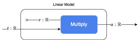
This is a function that constructs a linear model of the temperature anomaly data over time. A linear model is a model (i.e. a function that is a compressed representation of some data or process) that simply models the output as a rescaled version of the input. This string diagram takes a single input $ t $ for time, and it is of type $ \mathbb{R} $, which is the symbol for real numbers. Real numbers are the term in mathematics essentially for arbitrary decimal numbers like 4.10219 or -100.0003. In a programming language, real numbers would correspond most closely to floating point numbers. Real numbers are the most common type of numbers we will see, but sometimes we will deal with binary numbers or integers (which are the whole numbers like …-3, -2, -1, 0, 1, 2, 3…).

Our linear model takes a time (in years) represented by the variable $t$ and scales it by the parameter $r$ to produce the output $a$, that is, our linear function (model) is just $a(t) = r\cdot t$. A parameter is an input to the function or model that is fixed for some period of time, it does not freely vary like a variable such as $t$. I represent adjustable (also called trainable) parameters using the open circle at the end of the string. I represent fixed parameters using a solid circle at the end of the string (not yet depicted).

The parameter is also depicted as being enclosed inside the box of the linear model, suggesting that we have to do some work to open the box to modify it, whereas the input string $t$ can be freely changed with whatever input we want at any time.

In this case, you can think of $r$ like a simple conversion factor. Since $t$ is in years, $r$ would have the units $\frac{°C}{Years}$, such that the units cancel out to give us what we want, i.e. $a = \cancel{Year} \cdot \frac{°C}{\cancel{Year}} = °C\ (\text{anomaly})$. That is, $r$ tells us how many °C the temperature anomaly will increase (since $r$ is positive) per year; it is a rate of change.

Our linear model defines a line, so we want to choose a value for $r$ that makes the line model our data as best as possible. Let’s choose 2 points that seem to represent the data well at both ends.

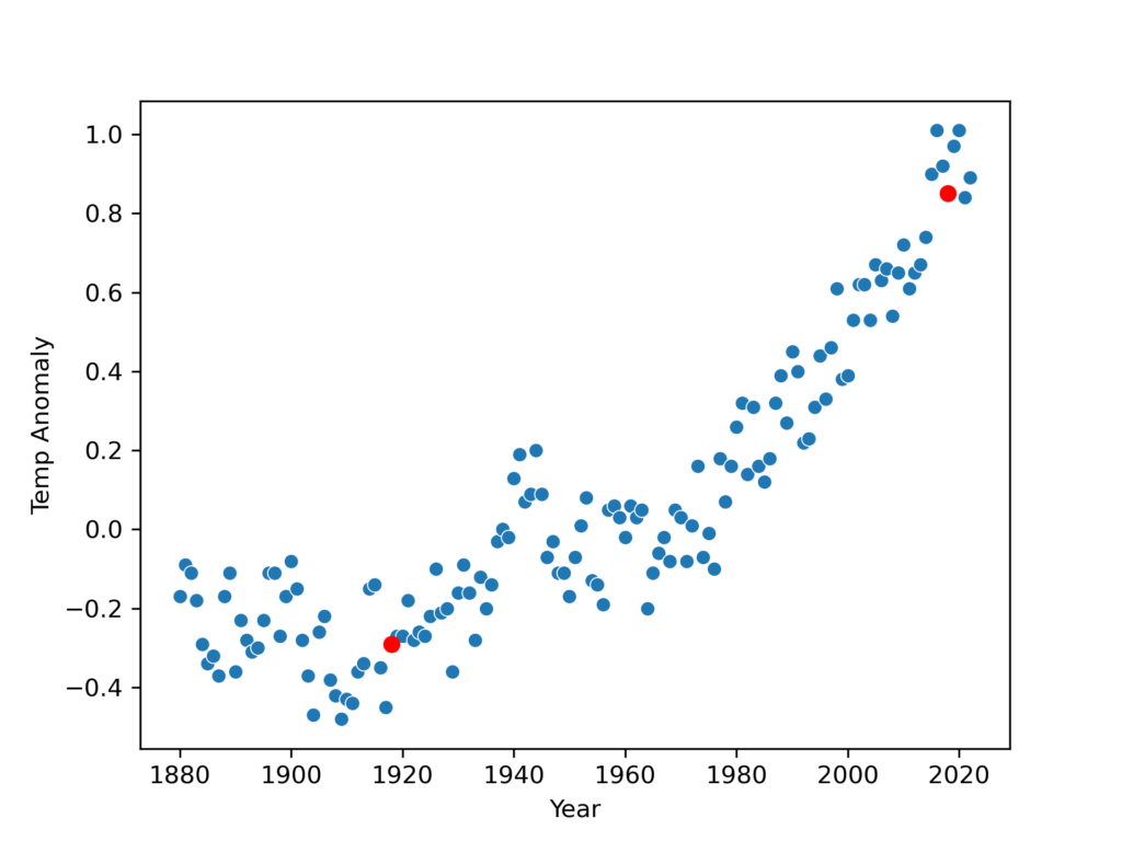
The points chosen were chosen just based on looking at this plot and selecting ones that appeared to represent the data near both ends. The point on the left, which we’ll all $p_1$, is at $(x = 1918, y = -0.29)$ and the point on the right, which we’ll call $p_2$, is at $(x = 2018, y = 0.85)$. Knowing these points, we can find the appropriate value for $r$.

$$\text{Line Slope} = \frac{y_2\ -\ y_1}{x_2\ -\ x_1}$$

$$ r = \frac{0.85\ -\ (-0.29)}{2018\ -\ 1918} = \frac{1.14}{100} = 0.0114$$

We’ve figured out the slope of the line, $r = 0.0114$, which fully determines our linear model, and means that for every 1 year increase in time, the temperature anomaly increases by 0.0114°C. So since in this dataset the last value recorded is for year 2022, with a measured temperature anomaly of 0.89, then we can predict on the basis of our linear model that in the year 2023 the temperature anomaly should be around $r + 0.89 = 0.0114 + 0.89 = 0.9014$.

But what if I want to predict the temperature anomaly for the year 2030? Well, if my last known value is $(year = 2022, a = 0.89)$, then 2030 represents 8 years in the future, so I need to add $r$ 8 times, hence, $(year = 2030, a = 8\cdot r + 0.89 = 0.9812)$. Having to figure out the difference in years and then multiplying that by $r$ is a little inconvenient, and this dataset will keep growing each year, so my last known value will change, meaning I have to change my calculation each time I want to predict out in the future. It would be better if I just had a function that takes in the year and spits out the predicted anomaly without reference to my last known data, like the string diagram I showed earlier.

We can do that, but we need to introduce an offset (also called, intercept, or bias in the machine learning context). See, as it stands now, knowing $r$ only tells us by how much the temperature anomaly will increase per 1 year, so to predict into the future we have to pick a changing reference point to add to. In order to get a nice function we can just plug any year in and get what we want, we need to have a fixed reference year. Let’s pick one of the two points we used to define our line as our fixed reference point, let’s choose $p_1 = (x = 1918, y = -0.29)$. It doesn’t matter which point we pick as long as it’s on our line.

Now we can make a new equation:

$$a = (y\ -\ 1918)\cdot 0.114\ -\ 0.29$$… which is of the more general form:

$$a = (y\ -\ y_{\text{ref}})\cdot r + a_{ref}$$, where $y_2$ is any year you want to input, $y_{\text{ref}}$ is the fixed reference year we choose, $r$ is our conversion rate (slope), and $a_{\text{ref}}$ is the temperature anomaly for the chosen $y_{\text{ref}}$ reference year. Now we can do a little algebra; let’s first distribute the $r$.

$$ a = r \cdot y\ -\ r \cdot y_{\text{ref}} + a_{\text{ref}} $$

Let’s substitute back in our values for $r, y_{\text{ref}}, $ and $a_{\text{ref}}$.

$$ a = 0.0114 \cdot y\ -\ 0.0114 \cdot 1918 + (-0.29) $$

This rearrangement allows us to separate out the terms involving the year $y$ and the fixed reference year $y_{\text{ref}}$ = 1918. Now, let’s combine the constants:

$$ a = 0.0114 \cdot y + (-0.0114 \cdot 1918\ -\ 0.29) $$

$$ a = 0.0114\cdot y\ -\ 22.1552 $$

Notice that the term $-0.0114 \cdot 1918 – 0.29 = -22.1552$ becomes our offset (aka intercept or bias), often denoted with the symbol $b$. This is the value of $a$ when $y = 0$, giving us the y-intercept of our linear equation. Thus, the function of our linear model is now in the same form as the grade-school equation for a line $y = mx + b$.

This new linear model with a fixed reference allows us to calculate the temperature anomaly $a$ for any year $y$, using a fixed reference point in time $y_{\text{ref}} = 1918$ and its associated temperature anomaly $a_{\text{ref}} = -0.29$, alongside our previously calculated rate of change, $r = 0.0114$.

Now we can add the line to the graph:

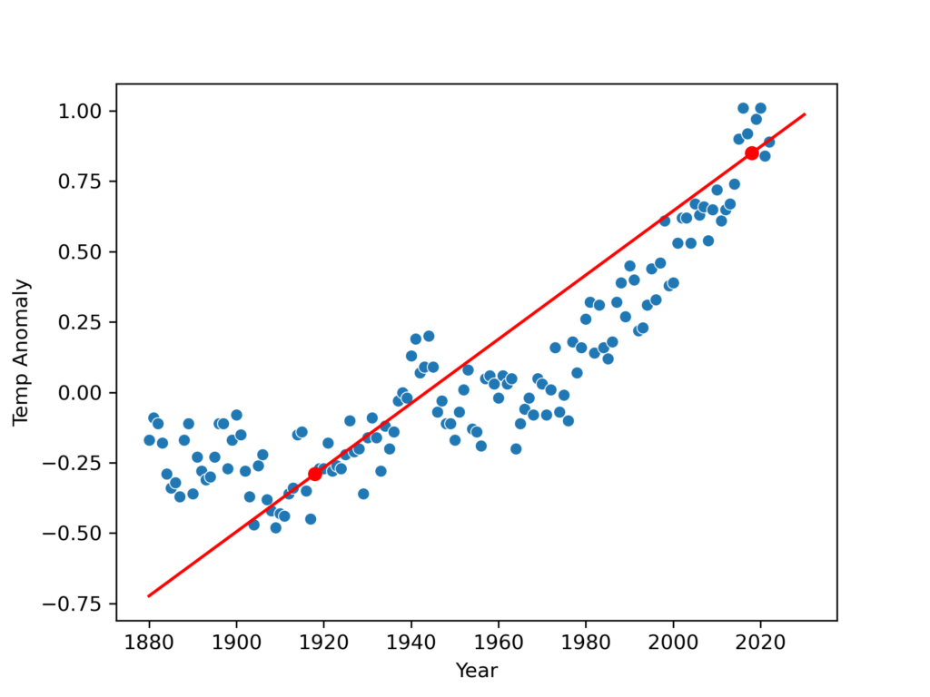
You can see our linear model doesn’t perfectly follow the data, mostly because the data is not perfectly linear, but it does a good enough job that we could probably use it to predict ballpark estimates of the temperature anomalies at least a few years into the future.

The Space of Data and Models

Our linear model takes a single number (the year) and returns a single number (the predicted temperature anomaly), and it basically has a single trainable or adjustable parameter, $r$, although the offset (aka intercept or bias) is also considered a parameter. So we have been working with one-dimensional data. When we speak of dimensions of data, we are first implicitly recognizing that data live in a mathematical space. A space in the mathematical and machine learning sense is a way of recognizing the distinctions between different data and how they relate. For example, here’s just a part of the temperature anomaly data as a sequence of numbers:

$$ [0.67, 0.74, 0.9 , 1.01, 0.92, 0.85, 0.97, 1.01, 0.84, 0.89] $$

Each number is the temperature anomaly for the years 2012-2022, in order. What can we say about the space that these data live in? Well, this space is composed of elements that are real numbers $\mathbb{R}$, which we introduced earlier. The elements of a space are like its atoms, it’s fundamental units (hence, elements being elemental). We also know that these elements have a temporal order, meaning we cannot just change the order, without disturbing the meaning of the data.

That leads me to perhaps the defining feature of a mathematical space:

A (mathematical) space is principally defined by what transformations (or moves) you can make in the space without fundamentally altering its meaning and structure.

A space’s structure is defined by how the data relate to each other. For example, if I were to change one data point from Celcius to Fahrenheit, then the meaning (i.e. semantics) of the space would not be changed (it is still a sequence of temperature anomalies over time), but the structure would be, since the difference in values would be quite large.

On the other hand, if I were to convert all of the values into Fahrenheit, then the meaning and structure would be preserved. To convert into Fahrenheit, all we have to do is apply a specific mathematical transformation to each data point. The formula for converting a temperature from Celsius to Fahrenheit is $F = C\cdot\frac{5}{9} + 32$, where $F$ is the temperature in Fahrenheit and $C$ is the temperature in Celsius. By applying this formula to each value in our sequence, we can convert the entire dataset to Fahrenheit.

This transformation would change the numerical values but not the relationships between them: the way one temperature anomaly compares to another over time — remain consistent. The overall pattern, trends, and differences between consecutive years are preserved. In essence, the data tell the same story, but in a different ‘language’ or unit.

As I alluded to earlier, these data live in a one-dimensional space, and that is because we can identify each data point by a single address number. For example, here’s our data again, but I’ve given it a name $T$:

$$ T = [0.67, 0.74, 0.9 , 1.01, 0.92, 0.85, 0.97, 1.01, 0.84, 0.89] $$

Now I can say that the value 0.74 lives at address 2 from the left, and we can access the value by using this notation: $T[2] = 0.74$. We will see later that spaces with more than one dimension will require more numbers to identify and access the data.

Just to hammer this point in, let’s enumerate some of the features of this space:

• The space can be uniformly scaled by a conversion factor (often called a scalar).
• A single number can be added to or subtracted from each value, which essentially shifts the temperatures up or down without disturbing the semantics or relationship between points.
• The space has a temporal order to it. We cannot move values around in the sequence arbitrarily.
• The distance between points in the space is taken by their absolute difference.
• We can course-grain the data by averaging over say 10 year blocks, which will not disturb the overall structure and semantics, it will just lower the resolution of the data.

Another way of thinking about a space is just like a type in a programming language with some constraints on what you can do with values of that type.

Let’s summarize what we’ve accomplished so far: We have built a linear model by choosing two representative points toward each end of the dataset and effectively drew a line through them to define our model. This linear model follows the trend of the data and thus could be used to predict future data. Is this a machine learning model? Arguably yes, it can be considered as a basic form of machine learning. Machine learning, at its core, is about creating models that can learn patterns from data and make predictions or decisions based on those patterns. Our linear model, although simple, does fit this description.

However, we as the human modeler were actively involved in “fitting” the model to our data. Usually when we think of machine learning models, there is an algorithm (aka procedure) that robotically figures out how to fit (aka train, or optimize) a particular model to the data, without us having to look at the data and do it ourselves. In this case, the training algorithm should automatically choose the conversion rate (slope) parameter $r$ and the offset parameter $b$ based on our data. There are a variety of training algorithms and we will learn how those work in more detail in another tutorial. In this tutorial, we will be manually training the models.

Vectors and Multidimensional Spaces

Our current linear model makes predictions about the future using only information about the past. We can likely get better performance (i.e. more accurate predictions) from our model if it uses additional data to make its predictions. We know that greenhouse gasses like carbon dioxide CO₂ in the atmosphere have an important impact on global average temperatures, so this seems like an important variable to include in our model.

Here’s what our new model looks like when it includes this additional input variable of average CO₂ concentration measured in parts per million:

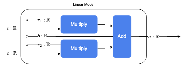
In mathematical notation this represents the function $\text{Predicted Temp Anomaly}(\text{time}, \text{CO}_2) = r_1 \cdot \text{time} + r_2\cdot \text{CO}_2 + b$, where the input $t$ is time (year), the input $c$ is CO₂ concentration in the atmosphere, $r_1$ and $r_2$ are scaling parameters and $b$ is the offset parameter.

In this case, the diagram looks more complicated than the function in standard math notation, but in the future you’ll see how these kinds of diagrams can communicate complex neural networks succinctly.

Okay, now we have a function with two inputs, which we’ve name $t$ (for time or year) and $c$ for CO₂. Since we cannot evaluate this function (i.e. run this program or process) until we have both inputs at the same time, it makes sense to package the two inputs into a pair $(t, c)$ rather than treat them as completely separate inputs. The more general form of a pair is an n-tuple, where a 3-tuple is something like $(a,b,c)$ where $a,b,c$ are all some type of input variables, and a 4-tuple is something like $(a,b,c,d)$, etcetera.

These n-tuples form what what is called a vector space in mathematics, and thus, the n-tuples are also called vectors that live in the vector space. The study of vectors and vector spaces is the domain of Linear Algebra, one of the most useful fields in mathematics. The known mathematical tools from Linear Algebra are critical to understanding and using neural networks.

Introduction to Linear Algebra

Recall, I previously introduced the concept of a mathematical space as a set of elements (or a type) and a set of allowable transformations (i.e. functions) on those elements (or values of the type) that preserve the structure and meaning (i.e. semantics) of the space. Well, a vector space is a space where the elements are called vectors and the allowable transformations between them are called linear transformations. Vector spaces, as mathematicians define them, are quite abstract and difficult to explain intuitively. Often vectors are introduced as arrows with magnitude and direction, and we will get to that, but in the most abstract and general case, even that is not accurate.

Vectors as displacements

A vector space encapsulates the idea of displacement. Displacement is simply the change from one state to another, for example, traveling 2 hours is a displacement in time, or traveling 2 miles North is a displacement in space, or making a \$500 deposit into your bank account is a displacement of money. Usually, displacements, unlike lengths or distances, have both a magnitude and an orientation (or direction). You can travel for +2 minutes, or you can rewind a video by 2 minutes, (i.e. the displacement being -2 minutes). You can go 2 miles north, south, east, west or any where in between. You can deposit money (e.g. +\$500) or withdraw money (e.g. -\$500). Vectors are displacements, and displacements are changes in state that usually have a size and an orientation.

In this sense vectors are conceptually different from “points” in a space. For example, 4:00 PM on a clock is a “point” in “time space.” It is a static reference point. But a vector like +2 hours can be added to the point 4 PM, moving us to the new point of 6 PM. Similarly, a specific location on a map is a point, and a vector might be “200 meters east,” such that we can add this vector to some point-like location and get a new location. Points in space do not inherently convey movement or change; they are static and absolute locations. It generally doesn’t make any sense to add static points in space, e.g. Tokyo + New York = ?, or 4 PM + 2 PM = ?.

Abstract vector spaces

Mathematically, vector spaces are defined as a set of elements, equivalently, a type with values (called vectors) such that you are allowed to add any two vectors and the sum will also be a vector in the set (or space or type), which is a property called closure. You are also allowed to scale up or down any vector by multiplying it by a number (called a scalar) and the result is also a vector in the same space, a property called scalar multiplication. There must also be a “zero vector” $\mathbb{0}$ such that for any vector $v$ in a vector space, $\mathbb{0} + v = v$, which is a property called additive identity. Thinking of vectors as actions, displacements or state changes, the zero vector is essentially the “do nothing” vector. Lastly, each vector $v$ in our vector space must have an additive inverse $-v$, such that $v + (-v) = \mathbb{0}$. Additive inverses are essentially “undo” or “reverse” vectors.

This is a very general and abstract definition and thus many things can qualify as a vector space. In fact, (real) numbers themselves qualify as a vector space, since you can add any two numbers and get another number and you can also multiply a number and you still get a number. And these numbers could semantically represent whatever you want, for example money in a bank account that can be added or withdrawn or scaled up (e.g. due to interest).

Families of functions can form a vector space, such as the set of polynomials $f_1(x) = x^2$ or $f_2(x) = 2x^3 + x$ because these kinds of functions can be added (e.g. $f_1 + f_2 = 2x^3 + x^2 + x$), scaled (e.g. $4 * f_1(x) = 4*x^2$), have additive inverses (e.g. $f_1 + -x^2 = 0$) and additive identity functions (e.g. if $f_0(x) = 0$, then $f_0 + f_1 = f_1$). Note how in this case each vector is in a sense an infinite object, since these function are defined over all real numbers from negative to positive infinity.

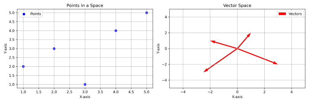
Most of the time in the machine learning context, we are dealing with vectors that are not that abstract and are just some numbers in a list, in which case we can think of these less abstract vectors as objects with direction and magnitude as opposed to points in space, which have a position (see figure 4).

Vectors in vector spaces can sometimes (depending on the context) be thought of as having multiple “components,” for example, like ingredients in a recipe. Consider the “space” of ingredients of cucumbers, sugar, sesame oil and soy sauce. Simply mixing these ingredients, in the proper proportions, can make a delicious and simple cucumber salad. Let’s represent these ingredients symbolically, such that $C$ = cucumbers, $S$ = sugar, $O$ = (sesame) oil, and $Y$ = soy sauce. Then we can say a particular recipe for this salad is the combination $a\cdot C + b\cdot O + c\cdot Y + d \cdot S$, where $a,b,c,d$ are numbers representing the amounts of each ingredient, e.g. number of cucumbers and tablespoons for the rest.

A specific recipe might be represented as $2C + 1O + 2Y + 1S$, signifying a recipe with 2 cucumbers, 1 tablespoon of sesame oil, 2 tablespoons of soy sauce, and 1 tablespoon of sugar (I removed the $\cdot$ symbol for brevity, i.e. $2C = 2\cdot C$). This is a vector in our vector space of cucumber salad recipes. We can more compactly represent this vector as simply an ordered list of numbers: $[2, 1, 2, 1]$ where each position represents the amount of cucumbers, oil, soy sauce, and sugar, respectively.

This space of ordered lists (aka 4-tuples) of numbers representing recipes constitutes a valid vector space because:

• Closure: The sum of any two recipe vectors (4-tuples) is another valid recipe vector in the space. For example, adding $[2, 1, 2, 1]$ (one recipe) to another, like $[1, 0.5, 1, 0.5]$, results in $[3, 1.5, 3, 1.5]$, which is still a valid recipe representation in this space.
• Scalar Multiplication: Multiplying a recipe vector by a scalar (a number) scales the quantities of each ingredient and results in another valid recipe vector. For instance, $2 \cdot [2, 1, 2, 1] = [4, 2, 4, 2]$. This is useful if we want to scale our serving size up or down.
• Additive Identity and Inverse: We have a zero vector $\mathbb{0}$, namely, $[0, 0, 0, 0]$ (meaning no ingredients; do nothing), which acts as the additive identity. And each vector has an additive inverse, allowing for ‘undoing’ a recipe, for example the vector $[-1, 0, 0, 0]$ corresponds to removing 1 cucumber. Remember, vectors are displacements so these vector recipes actually represent actions (not fixed states like points), e.g. the vector $[2, 1, 2, 1]$ means we add 2 cucumbers, 1 tablespoon of sesame oil, 2 tablespoons of soy sauce, and 1 tablespoon of sugar to our (presumably empty) bowl. Each component in the vector represents an action to be taken with a specific ingredient.

Each vector in this space represents a valid recipe, but not all of them are going to be tasty.

But notice, in order to set this up as a usable recipe, we had to choose specific units (e.g. tablespoons) to use for each ingredient. These choices represent a chosen basis for our vector space. In this recipe vector space, the basis vectors are the standard units (like one cucumber, one tablespoon of oil, etc.). Every possible cucumber salad recipe (vector) in this vector space can be described using a combination of our chosen basis vectors.

More mathematically, our basis vectors can be represented like this $[1,0,0,0], [0,1,0,0], [0,0,1,0], [0,0,0,1]$. Each basis vector represents a unit quantity of one ingredient while having zero quantities of the others. For example, $[1,0,0,0]$ represents adding one whole cucumber and no other ingredients. Similarly, $[0,1,0,0]$ represents adding one tablespoon of oil without any cucumbers, soy sauce, or sugar. Any valid salad recipe (vector) can be constructed by adding these basis vectors and multiplying them by scalars. For example, our first recipe of $[2, 1, 2, 1]$ can be seen as adding two units of the cucumber basis vector, one unit of the oil basis vector, two units of the soy sauce basis vector, and one unit of the sugar basis vector. In other words, it’s like $2 \cdot [1,0,0,0] + 1 \cdot [0,1,0,0] + 2 \cdot [0,0,1,0] + 1 \cdot [0,0,0,1]$. This demonstrates how any recipe in this vector space can be constructed using linear combinations of these basis vectors.

A linear combination of vectors is simply creating a new vector by adding and scaling two or more other vectors. For example, let’s say we have two vectors named $A$ and $B$, then we can linearly combine them to get a new vector $C = a\cdot A + b\cdot B$, where $a, b$ are scalars (numbers).

This leads naturally into a discussion of what exactly linear means in this context.

Linear versus Non-Linear

We touched on the idea of something being linear when we introduced linear models earlier. But the idea of linearity is quite deep and interesting. Generally, we use the term linear to describe a function (transformation). You might think a linear function is one that defines a line if we graph it, and that is true to an extant, but we want a notion of linearity that can work for functions in 3-dimensions, 4-dimensions, and beyond.

Let’s start with the mathematician’s definition of a linear function. Recall that a vector space is basically defined as a type where we have an add operation and a scalar multiplication operation, and nothing else. Well, a linear function is a function that preserves these two operations. Preservation, in this context, means that if you have a function that is linear, let’s call it $f$, and operations of $+$ and $\cdot$ (multiplication), then you get the same result whether you use $+$ and $\cdot$ first and then apply the function $f$ or if you apply the function $f$ first and then use $+$ and $\cdot$.

In mathematical terms, this means that a linear function $f$ satisfies the following equalities, given two arbitrary vectors we’ll call $u$ and $v$, and some scalar (number) called $a$.

$$ f(u + v) = f(u) + f(v) $$

$$ f(a\cdot u) = a\cdot f(u)$$

In other words, if we denote the $+$ and $\cdot$ operations in our vector space as functions and just call them say $t$ where $t$ could mean either $+$ or $\cdot$, then if a function $f$ is linear and we have an arbitrary vector $u$:
$$ f(t(u)) = t(f(u)) $$.

For example, the function $f(x) = 2\cdot x$ is linear because $f(2 + 3) = 10 = f(2) + f(3) = 4 + 6 = 10$.

Notice, however, that $f(x) = 2\cdot x + 1$ is actually not linear under this definition, despite it looking like a line when we graph this function, since $f(2 + 3) = 11 \neq f(2) + f(3) = 5 + 7 = 12$.

So if both $f(x) = 2\cdot x$ and $f(x) = 2\cdot x + 1$ look like straight lines when we graph them, why is only the former considered linear (in the context of linear algebra)? Well, because vector spaces capture the idea of a kind of conservation principle where you can’t get more out of a process than you put in.

Let’s pretend these simple functions are some sort of manufacturing processes that convert units of apples into units of applesauce. Our function $f$ is now some process take takes in some number of apples and turns them into some amount of applesauce.

$$f(x : \text{Apples}) = \frac{2\ \text{units of applesauce}}{1 \cancel{\text{apple}}} \cdot x \cancel{\text{apple}}$$

This looks very reasonable. You put in one apple and you get 2 units of applesauce (I leave the units unspecified here, maybe they’re cups or tablespoons or milliliters, it doesn’t matter). Also reasonable is the case if you put in 0 apples, you get 0 units of applesauce.

Now things get weird when we try our other linear-when-graphed-but-not-linear function:

$$f(x : \text{Apples}) = \frac{2\ \text{units of applesauce}}{1 \cancel{\text{apple}}} \cdot x \cancel{\text{apple}} + 1\ \text{unit of applesauce}$$.

If we put in 1 apple, we get 3 units of applesauce, more than the other function. Maybe this function is a more efficient way of producing applesauce, that’s certainly possible. But things get unreasonable when we put in 0. If we put in 0 apples, we will still get out 1 unit of applesauce. But how, where did this applesauce come from with no input apples? This process is apparently capable of producing applesauce out of nothing. That is what is non-linear about it. Linear functions don’t create stuff from nothing, 0 gets mapped to 0.

Let’s analyze another example function, say $f(x) = x\cdot x$, aka, $f(x) = x^2$. In terms of applesauce production, it could look like this:

$$f(x : \text{Apples}) = x^2 \cdot \frac{\text{1 unit of applesauce}}{\text{apples}^2}$$

If we put in 0 apples, we get 0 units of applesauce, so far so good. If we put in 1 apple, we get 1 unit of applesauce, if we put in 2 apples, we get 4 units of applesauce. Well if this was a linear applesauce maker, then if we put in 1 + 2 = 3 apples, we should get 1 + 4 = 5 units of applesauce. But we don’t, 3 apples in gets us 9 units of applesauce out.

Or more mathematically, $f(1 + 2) = f(3) = 3^2 = 9 \neq f(1) + f(2) = 1^2 + 2^2 = 1 + 4 = 5$. So this function does not preserve the vector space operations, so that is why it is not linear.

Overall, we care about vector spaces because they nicely capture types of things that can be added and scaled, and we care about linear functions (transformations) because they transform one vector space into another vector space by preserving the vector space operations.

Linear Transformations as Matrices

Linear Algebra is about vector spaces and linear transformations between vector spaces. Linear transformations are often represented as matrices.

A matrix is often introduced as a grid of numbers, like this:

A matrix in the mathematical / programming context is just a rectangular grid of values of some type (generally numbers). Matrices can be used in two different ways: 1) as a linear transformation and 2) as a data table. In machine learning, we will use both types of matrices, but for now, we will focus on matrices as linear transformations.

Recall, our recipe vector space from earlier had 4 ingredients denoted C (cucumbers), O (sesame oil), Y (soy sauce) and S (sugar). We decided that the units for C is number of cucumbers and the rest are measured in tablespoons. Let’s consider a set of linear functions on this recipe vector space that converts the measuring units into a different set of units. We’ll write some functions that convert everything into grams. We’ll need 4 functions, one for each ingredient.

$c \mapsto \frac{300\text{ grams}}{1\text{ cucumber}} \cdot c $

$ o \mapsto \frac{12\text{ grams}}{1\text{ tablespoon sesame oil}} \cdot o $

$ y \mapsto \frac{15\text{ grams}}{1\text{ tablespoon soy sauce}} \cdot y $

$ s \mapsto \frac{12\text{ grams}}{1\text{ tablespoon sugar}} \cdot s $

Note: I’ve used this new notation $\mapsto$ to define these functions without giving them names (just for convenience), called anonymous functions (also called lambda functions).

Now we can take any vector from the original recipe vector space, such as $(3,3,3,1)$ representing 3 cucumbers, 3 tablespoons of sesame oil, 3 tablespoons of soy sauce and 1 tablespoon of sugar, and convert it into a new vector space where all the ingredients are represented in terms of grams.

For example,

$c_{\text{new}} = \frac{300\ \text{grams}}{1\ \text{cucumber}} \cdot 3\ \text{cucumbers} = 900\ \text{grams}$

$o_{\text{new}} = \frac{12\ \text{grams}}{1\ \text{tablespoon sesame oil}} \cdot 3\ \text{tablespoons sesame oil} = 36\ \text{grams}$

$y_{\text{new}} = \frac{15\ \text{grams}}{1\ \text{tablespoon soy sauce}} \cdot 3\ \text{tablespoons soy sauce} = 45\ \text{grams}$

$s_{\text{new}} = \frac{12\ \text{grams}}{1\ \text{tablespoon sugar}} \cdot 1\ \text{tablespoon sugar} = 12\ \text{grams}$

So our new vector is $(900,36,45,12)$. This vector represents the same recipe, just in a new unit vector space.

Each of the conversion functions were linear functions and thus the overall transformation is linear as well. Notice each of these linear conversion functions has a single conversion factor number; we can package these up into a matrix. Here’s what the matrix representation looks like:

There are a bunch of zeros because the linear functions we made are not interdependent or interacting with each other. Each conversion function operates independently on its respective ingredient, without influencing the quantities of the other ingredients. The zeros in the matrix represent this lack of interaction or cross-dependency between different ingredients in the recipe. In other words, changing the amount of one ingredient (like cucumbers) does not affect how the amounts of the other ingredients (like sesame oil, soy sauce, sugar) are converted into grams.

If there were interactions, we could have made a linear function like this:

$c_{\text{new}} = m_1\cdot c + m_2\cdot o + m_3\cdot y + m_4\cdot s$

In this case, we have a function that returns a new number of cucumbers based on not just the current number of cucumbers but also the amount of the other ingredients.

This might represent a situation in which the recipe’s balance or taste profile is adjusted according to the quantities of the other ingredients. For instance:

• $m_1$ could still be the direct conversion factor for cucumbers, but…
• $m_2$ could represent how the amount of sesame oil influences the need for cucumbers (perhaps more oil reduces the need for cucumbers).
• $m_3$​ might show how soy sauce affects cucumber quantity (maybe more sauce complements fewer cucumbers).
• $m_4$​ could indicate a relationship between sugar and cucumbers (like more sugar balancing out the freshness of more cucumbers).

This reflects a more complex and interdependent relationship among ingredients than what is captured by simple unit conversions.

We could do the same for all the other ingredients, and then each ingredient would be converted into a new number by a linear combination (we learned about this earlier) of all the ingredients. Then for each ingredient we’d have 4 linear functions each with 4 scaling factors (also called coefficients), for a total of $4 \cdot 4 = 16$ coefficients. And recall, our matrix earlier had 4 rows and 4 columns.

To show how to use matrices, let’s first consider a simpler example.

This is a simple 2 x 2 matrix with entries labeled a, b, c, and d (representing some numbers). This matrix corresponds to two linear functions that transform a vector $X$ with components $x_1$ and $x_2$, i.e. $X = [x_1, x_2]$:

$ f_1(x_1, x_2) = y_1 = a\cdot x_1 + b\cdot x_2$

$ f_2(x_1, x_2) = y_2 = c\cdot x_1 + d\cdot x_2$

As a reminder, these functions are linear because each input (i.e. $x_1$ and $x_2$) is only scaled and added to a number, and hence preserves the vector space operations of plus and times.

Each one of these linear functions takes our input vector $X = [x_1, x_2]$ and produces a new component of an output vector we could call $Y = [y_1, y_2]$. Each linear function multiplies the input vector components with 2 numbers (aka coefficients, parameters, scalars) and then adds them together. By packaging these coefficients into the matrix we can define a recipe for how to use this matrix to achieve the same effect as using these 2 linear functions, namely, we define a procedure for how to multiply a matrix with a vector to get a new vector.

$$
M(X) = \begin{bmatrix} a & b \\ c & d \ \end{bmatrix} \begin{pmatrix} x_1 \\ x_2 \ \end{pmatrix} = \begin{pmatrix} a\cdot x_1 + b\cdot x_2 \\ c\cdot x_1 + d\cdot x_2 \ \end{pmatrix}
$$

To make this easier, let me first introduce the notion of the inner product or dot product of two vectors $a$ and $b$ is denoted $a \cdot b$ (note this is the same symbol for multiplication of numbers we’ve been using, but in this case these are vectors not just numbers), and is defined like this:

$$a \cdot b = \sum_{i=1}^{n}a_i\cdot b_i = a_0 \cdot b_0 + a_1 \cdot b_1 + … + a_n\cdot b_n$$

This is the common mathematical notation for adding (summing). It is basically a for-loop where we add the corresponding components of two lists of numbers.

Now that we’ve defined the dot product, matrix-vector multiplication can be explained as taking each row of the matrix $M$ and then taking its dot product with the vector. So for each row of the matrix we will get a new number. For a $2\times2$ matrix like $M$ above, we have 2 rows so we have 2 dot products yielding 2 new numbers, which form the components of a new vector.

Knowing this, we can write $M(X)$ in a different way:
$$ M(X) = y_i = M_i \cdot X $$

The vector that results from multiplying the matrix $M$ with vector $X$ is arbitarily called $Y$ but each of the two components is labeled $y_1$ and $y_2$ or $y_i$ more generally.

We call this notation indexing, which is a kind of addressing mechanism for vectors and matrices. A vector will have a single index which can take on values as long as the vector is. A matrix will have two indices since each value in the matrix has a corresponding row and column. There are also linear algebra types “beyond” matrices that have 3 or more indices (e.g. rows, columns, 3-D depth…) and we more generally refer to all of these as tensors. A 0-tensor is a single number (aka scalar), a 1-tensor is a vector, a 2-tensor is a matrix, and so on. The number indicates how many indices the tensor has.

So we can index (address) each row of the matrix $M$ but giving it an index $M_i$, where $i$ can be as any number as many rows as the matrix has, which is 2 in this case. So $M_1$ refers to the first row of the matrix. Thus each component $y_i$ is computed by taking the dot product between the corresponding row $M_i$ with the full 2-element vector $X$.

Notes:

Linear algebra is the field of mathematics that studies vectors and matrices, so we need to know a little bit about this area of math to understand neural networks.

A linear transformation (or linear function) is both very simple but also quite subtle in terms of how to make sense of its purpose. As such, we will take a few different perspectives of linear functions to attempt to understand them well.

Let’s first consider the example of a recipe to make

First, consider the number line:

Perspectives:

• abstract notion: additivity and scaling, axioms
• size and orientation (magnitude and direction)
  • a space/type characterized only by having a set of orientations (usually finite) and a set of sizes (unusually infinite)
  • f(x) = 0 is a linear function because it takes a vector space and returns a new vector space, which is just the set {0} (because scalar * 0 \in {0} and 0 + 0 \in {0}) whereas f(x) = 5 is not a linear function because it takes a valid vector space and transforms it into a non-vector space just the set {5}, since 2*5 \notin {5} and 5+5 \notin {5}.
  • no-cloning
  • uniformity / interpolatability ; by having a finite sample from the function you can determine the entire function
  • linear as most computationally efficient (number of data points needed to solve for the coefficients is 1 for a linear function or k for a polynomial of degree k)
  • dimensionality analysis and conservation principle (you cant get more out of the process than you put in) f(x: Apples) = 5 tablespoons / apple * x. f(x) = 0 is okay because it is like a process that can take in apples but doesn’t convert them at all into anything else. But f(x : Apples) = 5 : tablespoons is not allowed because you could get more juice out than you put apples. f(1) = 5 and f(2) = 5, where did the extra juice come from? I think thinking of the coefficient in the equations as being a dimensionful unit is helpful in motivating linearity as a resource-constraint. f(x,0) = f(x). f(x,5) != f(x). So f(x) = 5, in order to be linear, would need to be, f(x,y) = y, if y = 5. Basically we’re sneaking in the extra resources through a side channel.
  • The whole is equal to the sum of its parts
  • linear dynamical systems
  • linear logic: disallows deleting or duplicating premises
  • affine logic: only disallows duplicating premises, but allows deletion
  • vectors are displacements, points are locations (e.g. +4 hrs vs 4 pm)
  • A vector space represents an abstraction of the notion that “the whole is equal to the sum of its parts.” For example, if you take two glasses of water and combine (add) them, you get just another glass of water that is exactly equal to the sum of the two glasses of water in terms of volume, and otherwise shares all other properties. In contrast, if you consider H₂O water molecules, they are markedly different than the “sum” of the parts of hydrogen (a flammable gas) and oxygen (another gas). If H₂O as a whole was the sum of its parts (hydrogen and oxygen), we’d also expect it to be a flammable gas and oxidizer.
• I use the Principal Concepts Continuum (PCC) Method of teaching: Distill any difficult, complex subject into its most foundational (principal) concepts, and then teaching these concepts linearly along a continuum (as opposed to making large, discrete conceptual leaps) making the smallest conceptual steps as possible as you introduce new concepts.